Chapter 31 — Indifference Curves and Budget Lines
Cambridge International AS & A Level Economics (9708) · Unit 7.2 · 4th edition coursebook
Learning objectives
- Define the meaning of an indifference curve and a budget line.
- Explain the causes of a shift in the budget line.
- Analyse the income, substitution and price effects for normal, inferior and Giffen goods.
- Evaluate the limitations of the model of indifference curves.
Key terms
- indifference curve
- This shows all of the combinations of two goods that give a consumer equal satisfaction.
- marginal rate of substitution
- The rate at which a consumer is willing to substitute one good for another.
- budget line
- The combinations of two goods that can be purchased with given income and given prices.
- substitution effect
- Where, following a price change, a consumer will substitute the cheaper good for the one that is now relatively more expensive.
- income effect
- Where following a price change of a good, a consumer has higher real income and will purchase more of this good.
- Giffen good
- A type of inferior good where the quantity demanded falls as price falls and the quantity demanded increases as price increases.
31.1Indifference curves
Marginal utility theory shows that consumers buy more of a good when its price falls. But a price fall on its own is not enough — consumers will only buy more of a good if it is something they actually want or prefer relative to the available alternatives. The indifference curve model provides a different way of representing consumer preferences that does not require utility to be measured in numerical units. It works with rankings rather than amounts (see Figure 31.2).
An indifference curve shows all the combinations of two goods that give a consumer equal satisfaction. Along a single indifference curve the consumer is indifferent between every combination — each gives the same level of utility, so the consumer has no reason to prefer one over the other.
Properties of indifference curves
Indifference curves slope downwards from left to right. This is because if the consumer gives up some of one good, more of the other good must be added to keep total satisfaction the same. They are also conventionally drawn convex to the origin: as the consumer holds more of one good, they become increasingly willing to give up units of that good in exchange for the other. The rate at which a consumer is willing to give up one good for another is the marginal rate of substitution. Where consumption of good Y is large and consumption of good X is small, the consumer is willing to give up a lot of Y for a little extra X; where Y is scarce and X plentiful, the reverse applies. The slope therefore changes along the curve.
An indifference map is a diagram showing several indifference curves for the same consumer. Higher curves represent higher levels of satisfaction because they contain combinations with more of at least one good. A rational consumer will always prefer a higher indifference curve to a lower one. Indifference curves never cross — if they did, the consumer would be ranking two different levels of satisfaction as equal, which would be irrational and inconsistent with maximising satisfaction.

Indifference curves are convex to the origin because of a diminishing marginal rate of substitution: as the consumer holds more of one good, he is willing to give up less of it to obtain another unit of the other good. The slope therefore flattens along the curve, producing convexity - none of the other concepts explains the shape.
31.2Budget lines
Consumers are constrained by their disposable income and by the prices of the goods they buy. The budget line brings these two constraints together. It shows all the possible combinations of two goods that a consumer can buy with a given income at given prices. Every point on the budget line uses up the consumer's entire budget; combinations inside the line are affordable but leave income unspent, and combinations outside the line are unaffordable (see Figures 31.3 and 31.4).
Suppose a consumer has $200 to spend on goods X and Y, where the price of X is $10 and the price of Y is $20. The maximum quantity of X that can be bought (if no Y is purchased) is 20 units; the maximum quantity of Y is 10 units. A straight line joining these two intercepts shows every other affordable combination. Its slope reflects the relative prices of the two goods.
Causes of a shift in the budget line
The budget line moves whenever income or relative prices change.
If the price of one good changes while income and the other good's price are unchanged, the budget line pivots. Suppose the price of X falls. At every income level the consumer can now buy more X, so the X-intercept moves outwards. The Y-intercept does not move because the price of Y and income are unchanged, so the line pivots from its fixed point on the Y-axis. If the price of X were to rise instead, the X-intercept would pivot inwards.
When the price of X falls relative to Y, the rational consumer substitutes towards the good that has become relatively cheaper. This is the substitution effect. The price fall also raises the consumer's real income — the same money income now buys more — which may lead to additional purchases of X (and possibly Y). This is the income effect.
The effect of a change in income
The budget line and indifference curve can be used together to find the consumer's optimum choice. Consumer equilibrium occurs at the point where the budget line is tangent to the highest indifference curve the consumer can reach. At this tangency point the slope of the indifference curve (the marginal rate of substitution) equals the slope of the budget line (the relative price), so the consumer cannot reach a higher curve given the budget.
A rise in income shifts the budget line outwards in a parallel way (relative prices are unchanged) and allows the consumer to reach a higher indifference curve. Where both goods are normal goods, consumption of each rises, although possibly to a different extent. If an increase in income causes consumption of a good to fall, that good is an inferior good. A fall in income shifts the budget line inwards in a parallel way, reducing consumption of both normal goods.
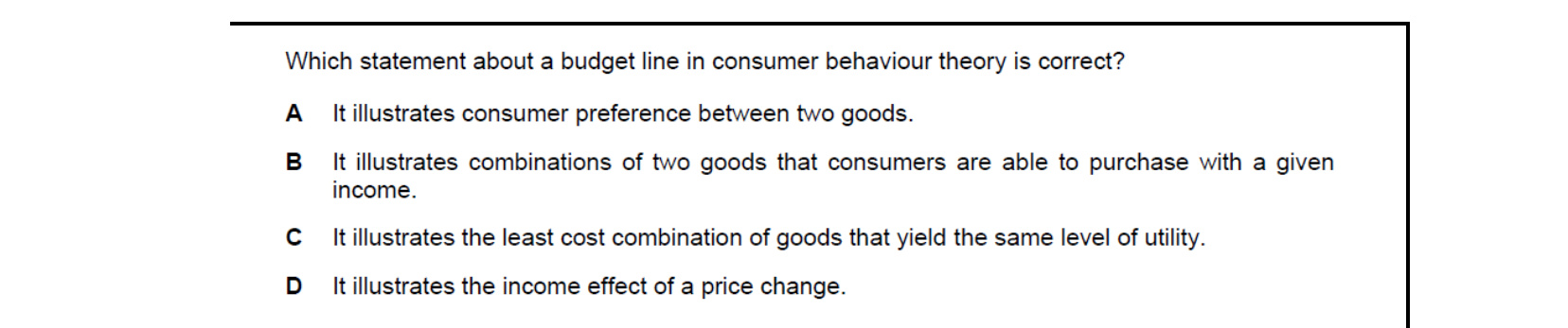
A budget line shows the bundles of two goods a consumer can afford given income and prices. It is determined by the constraint p(X)X + p(Y)Y = income, so it represents combinations of two goods that consumers are able to purchase with a given income. Preferences are shown by indifference curves, not by the budget line.
31.3The income and substitution effects of a price change
Indifference curve analysis decomposes the effect of a price change into two distinct parts: a substitution effect and an income effect. The substitution effect captures the change in consumption that arises purely because relative prices have changed; the income effect captures the change that arises because real purchasing power has changed (see Figures 31.5, 31.6 and 31.7).
To isolate the substitution effect, an imaginary budget line is drawn parallel to the new budget line but tangential to the original indifference curve. The movement along the original indifference curve, from the initial equilibrium to the tangency with the imaginary line, is the substitution effect. The further movement to the new equilibrium on a different indifference curve is the income effect.
An increase in the price of a normal good
When the price of good X rises, the budget line pivots inwards on the Y-axis. The consumer can no longer reach the original indifference curve. The substitution effect is a movement along the original indifference curve: consumption of X falls because X is now relatively more expensive than Y. The income effect is a shift to a lower indifference curve because real income has fallen; for a normal good this effect also reduces consumption of X. Both effects therefore work in the same direction and X consumption falls unambiguously.
A decrease in the price of a normal good
When the price of good X falls, the budget line pivots outwards on the Y-axis. The substitution effect raises consumption of X because X is now relatively cheaper than Y. The income effect is positive — real income has risen and X is normal — so consumption of X rises further. The two effects reinforce each other and X consumption rises.
The case of an inferior good
For an inferior good the income effect works in the opposite direction to the substitution effect. When the price of an inferior good X falls, the substitution effect raises consumption of X (consumers substitute towards the cheaper good), but the rise in real income causes consumers to switch towards more expensive, higher-quality substitutes. The income effect is therefore negative. Provided the negative income effect is smaller than the positive substitution effect, consumption of X still rises overall and the demand curve still slopes downwards.
The case of a Giffen good
A Giffen good is a special type of inferior good. It is typically a staple food item that takes up a large share of low-income consumers' spending — rice or wheat flour are commonly cited examples. When the price of the staple food rises, real income falls so sharply that consumers can no longer afford the more expensive alternatives they previously combined with the staple. They therefore consume more of the staple, not less. The negative income effect is larger than the positive substitution effect, so quantity demanded rises as price rises. The reverse occurs when the price of the staple falls: real income rises, consumers switch towards other foods, and demand for the staple falls. The demand curve for a Giffen good slopes upwards.
Key concept link — The margin and decision-making
The use of indifference curves and budget lines are relevant examples of how decision-making by individuals is based on choices at the margin.
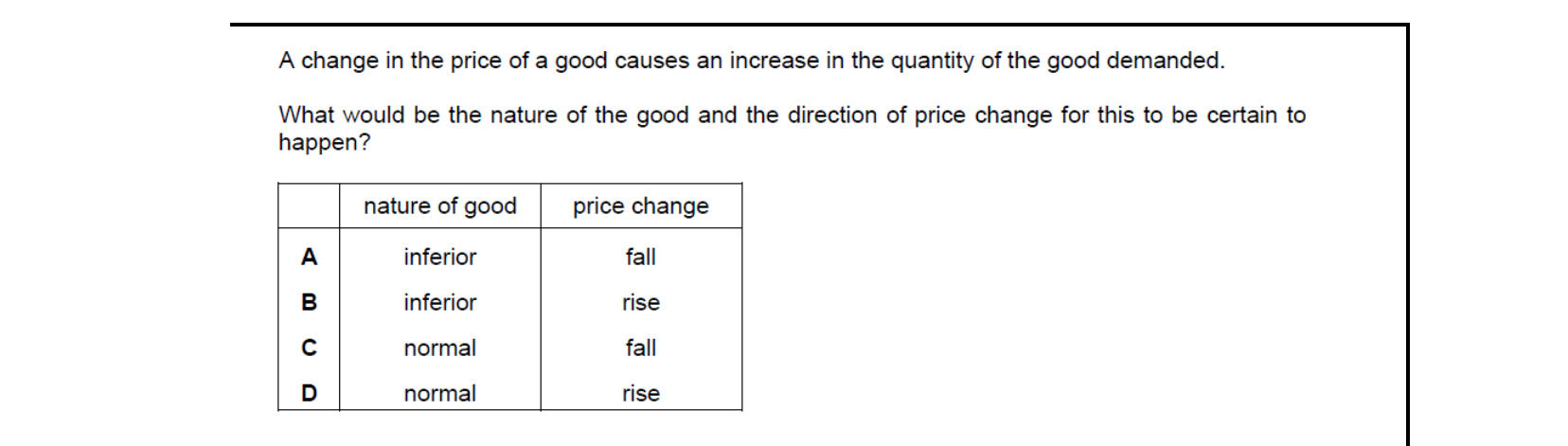
Demand certainly rises when price falls only when both the substitution and income effects raise quantity demanded. A normal good with a price fall gives a positive substitution effect and a positive income effect (real income rises and consumption of a normal good rises), so the increase is certain. With an inferior good the income effect opposes the substitution effect, so the outcome is ambiguous - hence normal good, price fall.
31.4Limitations of the model of indifference curves
The indifference curve model is a simplified representation of consumer choice. The analysis above has assumed there are only two goods and a fixed income, which keeps the model tractable but limits its realism. Three main limitations should be recognised.
- Real consumers choose between far more than two goods. A single visit to a supermarket may involve hundreds of products. A two-good diagram cannot capture this complexity.
- The word 'indifference' implies that the consumer is genuinely willing to accept any combination of two goods that lies on a given indifference curve. Some economists object that consumers actually express their wants as preferences or rankings, not as indifference between bundles.
- The model assumes consumers behave rationally — that they always choose the affordable combination that lies on the highest indifference curve. As Chapter 30 noted, real behaviour is shaped by many influences other than utility maximisation, so this assumption does not always hold.
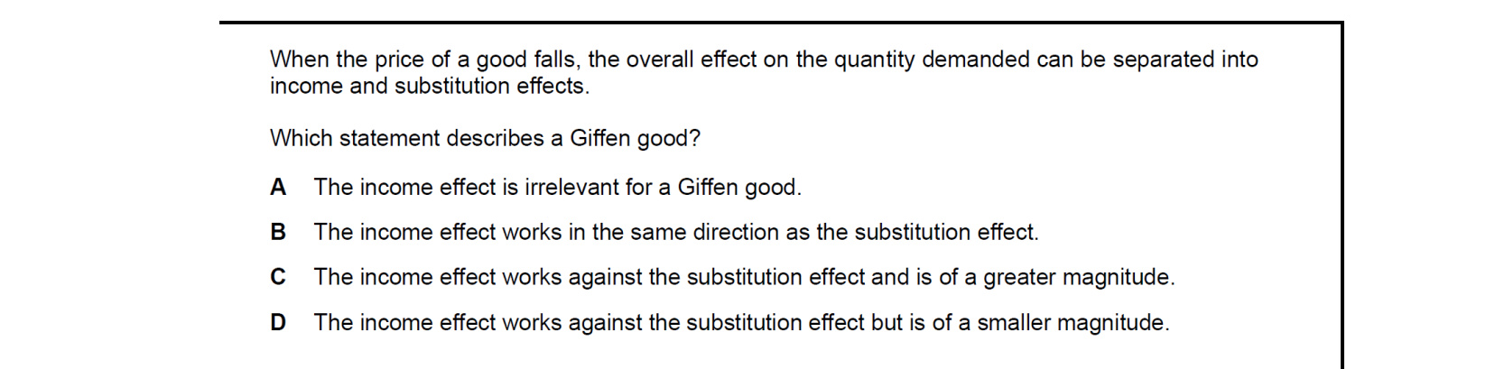
For a Giffen good, demand rises when price rises. The substitution effect of a price rise reduces demand, so the income effect must work in the opposite direction (raising demand) and outweigh it. This requires the good to be inferior and to take up a large share of income, so the income effect works against the substitution effect and is of a greater magnitude.
End-of-chapter practice
Past-paper questions from CIE 9708. Pick A, B, C or D. Answers are saved on this device — press Download report (PDF) at the top to save them.
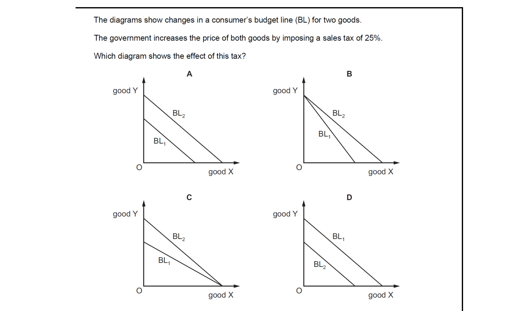
A 25% sales tax raises the price of both goods by the same proportion, so the consumer can buy 20% less of each good with the same income. Both intercepts of the budget line move inwards by the same proportion, producing a parallel inward shift. The diagram showing a parallel inward shift of the budget line is the correct one.
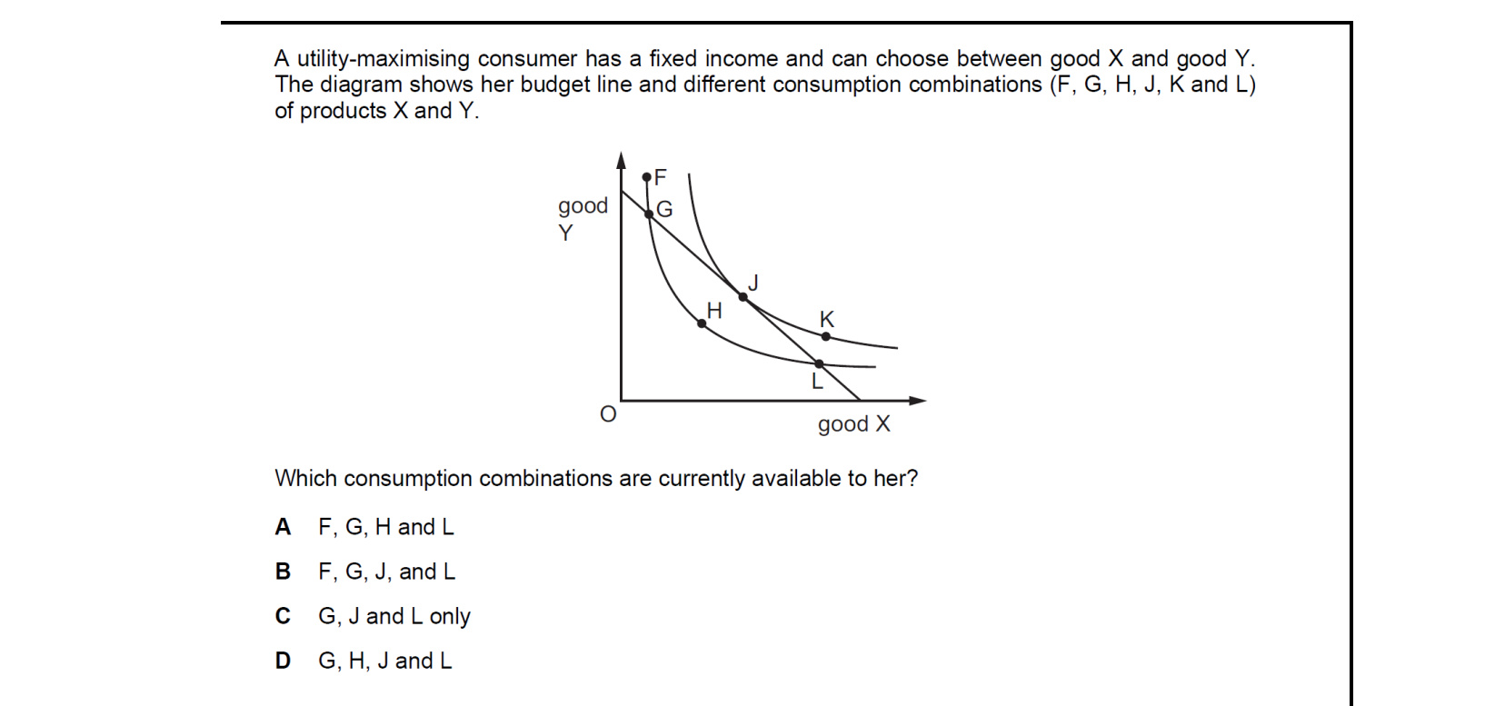
All affordable combinations lie on or inside the budget line. Points on the line use the whole income, while points inside it leave some income unspent; points outside it are unaffordable. The option listing only the bundles on or inside the budget line - G, H, J and L - identifies all currently available combinations.
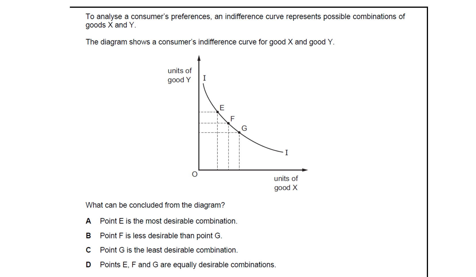
Every point on a single indifference curve gives the consumer the same level of total utility. Since E, F and G all lie on the same indifference curve in the diagram, the consumer is indifferent between them - points E, F and G are equally desirable combinations.
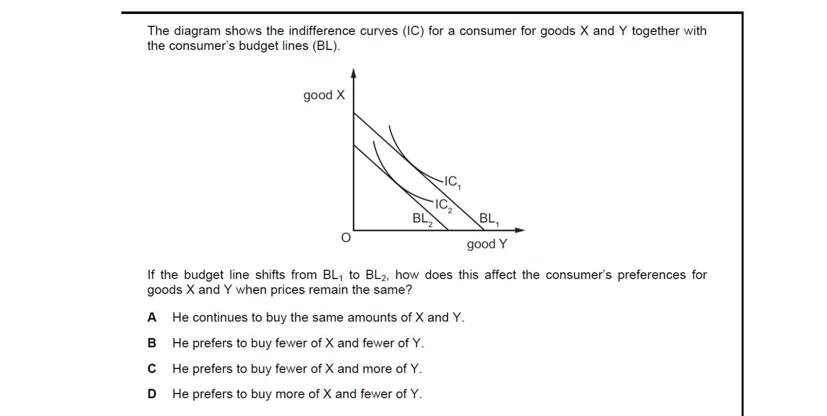
The new budget line BL2 lies entirely inside BL1 in parallel, so prices are unchanged but income has fallen. The consumer's new equilibrium is at the tangency on a lower indifference curve, which in the diagram lies at a position with less of both goods. So the consumer prefers to buy fewer of X and fewer of Y.

When the price of good X falls, the budget line pivots outward along the X-axis and the new tangency lies on a higher indifference curve with more of X consumed. Tracing the price-consumption path gives the demand curve for X with a normal downward slope. The matching diagram is the standard downward-sloping demand curve for good X.
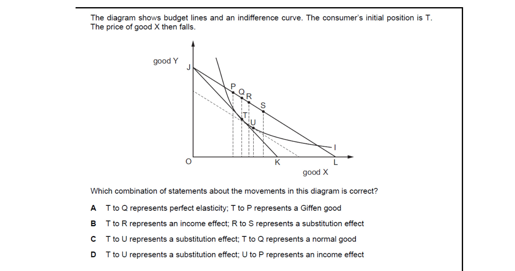
Following Hicksian decomposition, a hypothetical budget line tangent to the original indifference curve isolates the substitution effect (T to U), while the parallel shift to the new actual budget line gives the income effect (U to P). So T to U is the substitution effect and U to P is the income effect - the correct pairing.
Attempt the practice questions above to build your score.
Self-evaluation checklist
After studying this chapter, you should be able to:
- Understand that an indifference curve shows the combinations of two goods that give a consumer equal satisfaction.
- Understand that a budget line shows the combinations of two goods that can be purchased with a given income and prices.
- Explain why a change in price of one good will result in a shift in the budget line.
- Analyse the income, substitution and price effects for normal, inferior and Giffen goods.
- Evaluate the limitations of the model of indifference curves.
Want more practice? Drill this chapter's past-paper MCQs (88 questions) →